
NLP and Application: MBTI Personality Prediction
Date:
We tried different model in machine learning to develop a classifier capable of predicting an individual’s MBTI personality type based on text inputs, such as social media posts.
DATASET DESCRIPTION
The MBTI dataset can be downloaded publicly on the website of Kaggle. It’s originally scrapped form a website called “Personality Cafe”. The dataset contains 8675 inputs form different users. Each input consists of 50 recent comments from a user and each user is labeled the corresponding MBTI type. 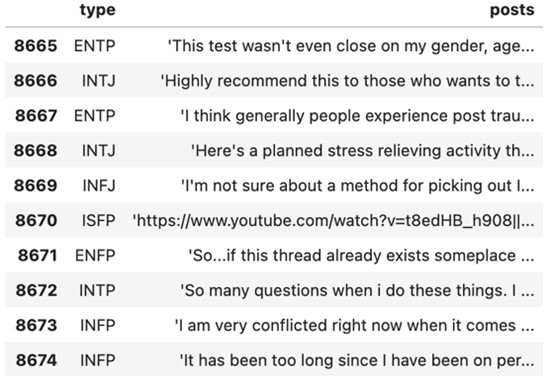
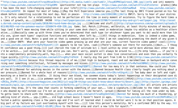
Form the first post we can find that each comment is separated by “|||”, and some comments contains URL links and repeated punctuation marks, which we considered meaningless.
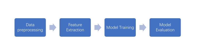
DATA PRE-PROCESSING
- Data Cleaning
Firstly, since the data was obtained from online platform comments, it is obviously that users often incorporate symbols to form text emoticons or random combinations of numbers and symbols, such as “:)”. These expressions are challenging for machines to comprehend, so we opt to remove them from the data. Secondly, users sometimes include image or video links within their comments, which represent as hyperlinks in the data set. Consequently, we replace these hyperlinks with spaces. Thirdly, in English text, certain words are extremely common but typically lack substantial meaning. These words, such as stopwords (e.g., “a,” “the,” “or”), can be disregarded for analysis purposes. To accomplish this, we utilize the stopwords corpus by NLTK to eliminate them from the data. Lastly, there are instances where words may possess different spellings while conveying identical or similar meanings. For instance, “apple” and “apples,” “is” and “was.” To facilitate model training, we employ the WordNetLemmatizer from NLTK to lemmatize words to their base or dictionary form (lemmatization) within the text.
There are some questions that deserve discussion:
1.Whether to retain punctuation marks:
There is a valid reason to consider the impact of punctuation marks on determining MBTI types. Individuals with a “Judging” personality type are likely to ask more questions compared to those with a “Feeling” personality type. Taking this into consideration, in the final model, I will attempt to replace various punctuation marks with specific English words, such as replacing “?” with “questmark”, to examine whether it improves the overall accuracy.
2.Whether to remove MBTI vocabulary:

Word cloud of posts from INFJ
Based on word clouds, it is evident that users of different MBTI types tend to mention their own personalities in their discussions. This means that these individuals have already implied their MBTI in the text. Intuitively, retaining MBTI vocabulary could potentially improve the prediction accuracy. However, one concern is that if the model assigns high weights to these specific MBTI-related words, what happens when there are instances where certain samples mention MBTI terms that do not align with their actual types? Could this potentially mislead the final prediction results? To investigate this issue, I will use the final model to evaluate different approaches to data cleaning. This will help determine the optimal method for handling MBTI vocabulary and its impact on the accuracy of predictions.
- Feature Engineering
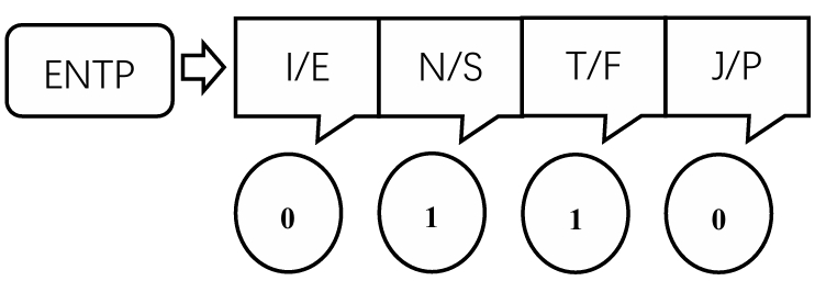
In this study, our target variable is the MBTI type. Since we need to predict each of the four dimensions separately, I have added four additional variables to the original data, each corresponding to one of the four dimensions.
In terms of input feature extraction, we use TF-IDF (Term Frequency-Inverse Document Frequency) to represent the importance of a term in a corpus. TF-IDF combines two components: term frequency (TF) and inverse document frequency (IDF).
Term Frequency (TF) measures the frequency of a term within a document. It indicates how often a word appears in a specific document relative to the total number of words in that document.
TF = (Number of occurrences of term ‘t’ in document ‘d’) / (Total number of terms in document ‘d’)
\[\mathbf{TF =}\frac{\mathbf{n}}{\mathbf{N}}\]Inverse Document Frequency (IDF) measures the importance of a term in a corpus. It quantifies how rare or common a term is across all documents in the corpus.
IDF = log ((Total number of documents) / (Number of documents containing term ‘t’))
\[\mathbf{IDF = log}\frac{\mathbf{N}}{\mathbf{n + 1}}\]The TF-IDF score of a term in a document is obtained by multiplying the term’s TF by its IDF. The higher the TF-IDF score of a term in a document, the more relevant or important the term is to that document.
TF-IDF = TF * IDF
- Train-test Spilt
This research uses 80% of the data for training and 20% for test.
METHODOLOGY
- Model Specification
This paper investigates five machine learning methods for classification: Logistic regression (Logit), Gaussian Native Bayes (GNB), K-Nearest Neighbors (KNN). Random Forest (RF), Support Vector Machines Classification (SVC)
- Cross Validation
We use 5-fold cross validation. That is, each model was trained on subsets for 5 times. “RandomizedSearchCV” is used to find the best hyperparameters for models with hyperparameters.
A visualization of how to find best k in KNN

A visualization of how to find best depth in DT
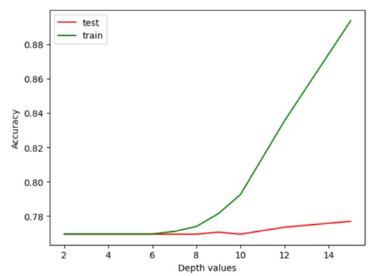
Below is the specification imposed on the 4 model with hyperparameters in this paper.
Logistic Regression (Logit)
(a). C: [0.01, 0.1, 1, 10, 100]
(b). solver: [lbfgs, liblinear, sag, saga]
(c). class_weight: [balanced, None]
K Nearest Neighbor (KNN)
(a). Numbers of neighbor: [3, 4, 5 … 26]
(b). Weights: [Uniform, Distance]
(c) Metric: [Euclidean, Manhattan]
Random Forest (RF)
(a). Numbers of estimators: [100, 200, 300]
(b). Maximum depth: [2, 3, 4 … 15]
Support Vector Machines (SVC)
(a). C: [0.1, 1, 10]
(b). gamma: [0.1, 0.01, 0.001]
(c). kernel: [rbf, linear, poly]
- Performance Evaluation
Below are confusion matrices for I/E Prediction
| I/E Prediction | Predicted I | Predicted E |
|---|---|---|
| Actual I | True Positives (TP) | False Negatives (FN) |
| Actual E | False Positives (FP) | True Negatives (TN) |
RESULT & EVALUATION
| Accuracy (out sample test) | |||||
|---|---|---|---|---|---|
| I/E | N/S | T/F | J/P | Overall | |
| Logit | 0.848 | 0.904 | 0.863 | 0.797 | 0.527 |
| GNB | 0.711 | 0.788 | 0.782 | 0.681 | 0.298 |
| KNN | 0.832 | 0.886 | 0.714 | 0.725 | 0.382 |
| RF | 0.778 | 0.862 | 0.828 | 0.656 | 0.364 |
| SVC | 0.862 | 0.904 | 0.866 | 0.786 | 0.534 |
| F1 score | Training time | ||||
| I/E | N/S | T/F | J/P | ||
| Logit | 0.904 | 0.946 | 0.851 | 0.733 | 6 min |
| GNB | 0.797 | 0.869 | 0.763 | 0.607 | 2 s |
| KNN | 0.900 | 0.937 | 0.595 | 0.537 | 102 s |
| RF | 0.874 | 0.926 | 0.803 | 0.258 | 5 min |
| SVC | 0.907 | 0.946 | 0.856 | 0.702 | 63 min |
Comparing the accuracy and F1 scores of all models, it is not surprising that the Naive Bayes model performs poorly in all four dimensions. This is because the Naive Bayes model is based on the assumption of feature independence, while in actual data, there is some correlation among the features, especially in the case of language vocabulary. The overall accuracy is 29.8%.
The SVC performs well in most dimensions. Since our post-processed data have very high dimensions, SVC’s superior performance can be attributed to its capability to construct intricate decision boundaries in high-dimensional space. By leveraging kernel functions, SVC can effectively map data onto higher-dimensional feature spaces, where it can identify non-linear patterns and achieve better classification accuracy.
All the models do not perform well in the F/T dimension and J/P dimension; However, data in these two dimensions are more balanced. The problem might be that data imbalance can lead to upward bias: When one class has a significantly larger number of samples than the other classes in the dataset, the classifier may tend to classify samples into the majority class. In this case, the classifier’s accuracy in I/E and N/S may appear higher because the majority of class samples are correctly classified most of the time.